Tuning Methodology
Contents
Methodology
- 1. List tables in query
- 2. List the joins in the query
- 3. Layout a diagram tables as nodes
- 4. Draw connectors for each join in where clause
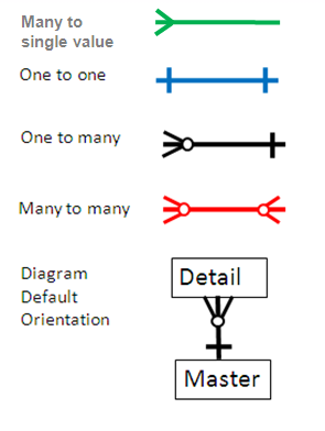
- 1 to 1 connection
- use blue line
- 1 to many
- use black line
- crows feet towards many
- many to many
- crows feet on both ends
- 5. Calculate filter ratios for any tables with filters
- filter ratio = number of rows returned with fitler / number of rows
- display in yellow below table node
- 6. Calculate two table join sizes for all two table joins in diagram (ie for every connection line)
- extract the join information, including filters, and run count on that join
- display in red on join line
- Alternatively, or as a complement, calculate join filter ratios in both directions
- display at each end of join connection line
- 7. Find the table sizes for each table
- display in green above table node
- Here is a query from Dan Tow's "SQL Tuning" which was the foundation for much of the ideas here:
- SELECT C.Phone_Number, C.Honorific, C.First_Name, C.Last_Name,
- C.Suffix, C.Address_ID, A.Address_ID, A.Street_Address_Line1,
- A.Street_Address_Line2, A.City_Name, A.State_Abbreviation,
- A.ZIP_Code, OD.Deferred_Shipment_Date, OD.Item_Count,
- ODT.Text, OT.Text, P.Product_Description, S.Shipment_Date
- FROM Orders O, Order_Details OD, Products P, Customers C, Shipments S,
- Addresses A, Code_Translations ODT, Code_Translations OT
- WHERE UPPER(C.Last_Name) LIKE :Last_Name||'%'
- AND UPPER(C.First_Name) LIKE :First_Name||'%'
- AND OD.Order_ID = O.Order_ID
- AND O.Customer_ID = C.Customer_ID
- AND OD.Product_ID = P.Product_ID(+)
- AND OD.Shipment_ID = S.Shipment_ID(+)
- AND S.Address_ID = A.Address_ID(+)
- AND O.Status_Code = OT.Code
- AND OT.Code_Type = 'ORDER_STATUS'
- AND OD.Status_Code = ODT.Code
- AND ODT.Code_Type = 'ORDER_DETAIL_STATUS'
- AND O.Order_Date > :Now - 366
- ORDER BY C.Customer_ID, O.Order_ID DESC, S.Shipment_ID, OD.Order_Detail_ID;
- SELECT C.Phone_Number, C.Honorific, C.First_Name, C.Last_Name,
Step 1 : Tables
- List tables in the query, for example from the query above
- Orders O,
- Order_Details OD,
- Products P,
- Customers C,
- Shipments S,
- Addresses A,
- Code_Translations ODT,
- Code_Translations OT
Step 2 : Joins
- Identify all the joins in the query, for example from the query above
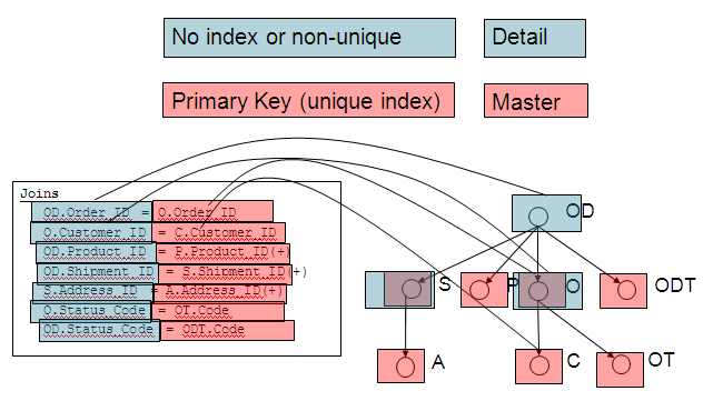
- OD.Order_ID = O.Order_ID
- O.Customer_ID = C.Customer_ID
- OD.Product_ID = P.Product_ID(+)
- OD.Shipment_ID = S.Shipment_ID(+)
- S.Address_ID = A.Address_ID(+)
- O.Status_Code = OT.Code
- OD.Status_Code = ODT.Code
Step 3: Laying Out Join Diagram
- Lay out the tables in the query as nodes, with a line connecting each table that is joined.
- What kind of method do we have for laying out the join diagram?
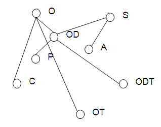
- Laying the out willy nilly is mostly a mess:
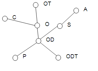
- Laying the out in a balanced tree could be of some use:
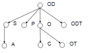
- but the real power comes in when we start laying them out with join relationships as our guide:
we put details above masters. Some masters are actually the detail for other masters.
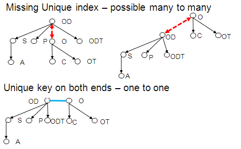
This structure will first of all quickly indicate any schema irregularities such as Cartesian joins (no join) , implied Cartesian joins (two details for one master), many to many relationships(potential exploding joins) and one to one relationships(ok sometimes but worth questioning the reasoning).
OK, so the diagram tells me some nifty things about the schema and relationships but you say "that's a lot of work for just some nifty stuff especially if I have to do it by hand and it's not automated." well, first it is automated in DB Optimizer and second there's a lot more we can do with the VST diagrams. First of all the diagrams give us a sense of what's happening in the diagram and tells us how information about the impact will have on the running row set. The running row set is the amount of rows that result from a starting join and that we carry to the next table that we join and so on until we finish all the joins in the query. Joining up in the diagram typically expands the running row set where as joining down typically keeps running row set the same:
Step 4: Join Connectors
Step 5: Predicate Filter Ratio
- In order to find the optimal path through the join tree we need one other thing - the predicate filter ratio. The predicate filter ratio is the fraction of the table returned after applying any restrictions in the where clause other than the joins. For example:
- select v.green, f.yellow from vegetables v, fruit f where f.blue=v.blue and f.red='1000';
- the where clause phrase f.red='1000' is a predicate filter. The predicate filter ratio, or filter ratio is the
- (select count(*) from fruit f where f.red='1000') / (select count(*) from fruit)
- Basically the table with the most selective filter is where we want to start the query and we want to go to the next most selective.
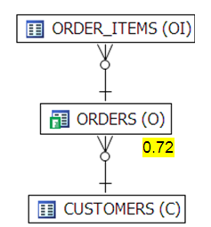
- Here is an example query from "swingbench" a load simulation tool for Oracle:
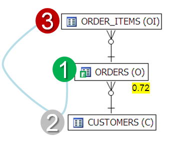
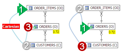
- It's clear that the execution path should be:
Because there is only one filter, the "0.72" on Orders. We join down from there to Customers then up to Order_Items.
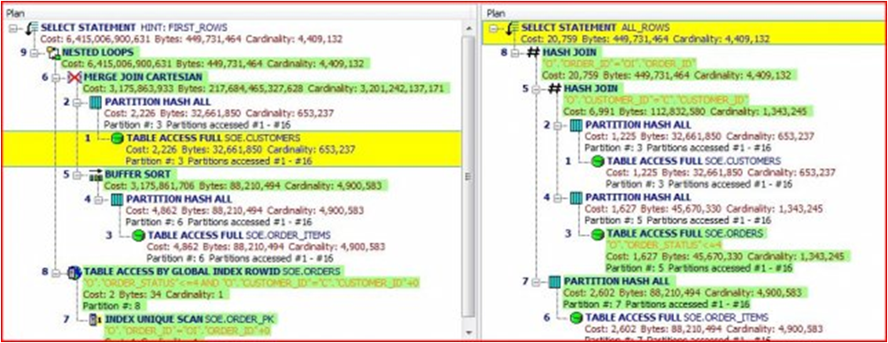
Now compare this to old style execution plans. Below is a comparison of two possible execution plans on the same query shown side by side:
First it difficult to read the information, second it takes time to load up enough of the information in to the mind and then play with it enough to understand what's happening and finally it's difficult to see whether these plans are realistic or not.
The above image shows the comparison of two alternative execution plans on a SQL statement. The text version on the left is the classic "explain plan" compared side by side. The right side is the same information but shown graphically. The Green Arrow labeled "1" is where the plan starts, followed by 2 then ending at 3. The joins are labeled "HJ" for hash join and "MJ" for merge join. The tables are ordered themselves not by execution order but by their relationship with details located above masters. The most important information is the join order. Of secondary interest is the join type, merge join, hash join or nested loops.
What I'm working on right now is making Explain Plans easier. Compare the textual explain to the graphic one. The graphic is so much easier. At the font size the text version is impossible top read. Even if it was big enough, the text would still take longer and more brain CPU cycles to understand. The graphic on the right tells me the most important information to optimally execute the query. The query will be optimally executed by starting on Orders, since it is the only table with a filter on it represented by both the little green F 9we will increase the size in the next version of DB Optimizer to make it more obvious) and the highlighted yellow "0.72". The value "0.72" is the filter ratio, or the fraction of rows returned after applying the query filters on this table. The filter "0.72" is the only filter ratio in the diagram, but if there was another filter ratio, we would pick the most selective one as the table to start are query, but in this case there is only one filter. From that filter we always join down into mater tables (master tales have the cross end of the join line - the crows feet represents detail table). By joining into a master table we keeps the same size of the "running row set" . The "running row set" the internal number of rows that are carried from one join to another as we join into each table in the execution plan. Can you imagine having carry boxes to 3 people in the office but depending on the order you visited the 3 people you either got to drop off boxes or you had to pick up boxes. Then the easiest most effortless path would be the path where you got rid of the most boxes first and picked up the least number of extra boxes along the way. The number of boxes you have to carry is equivalent to the running row set. For example in the above executions paths that are being compared, the one on the left does a join between ORDER_ITEMS and CUSTOMERS but there is no join so instead of getting rid of boxes we multiply - we do a Cartesian join. Thus this plan is not worth pursuing. The second plan is not worth pursuing because it joins from a master into a detail again increasing running row count prematurely - not as bad as a Cartesian but still worse than joining down to the master.
Step 6: Two Table Join Sizes and Join Filters
- Join diagrams with the relationships and predicate filter ratios can take us a long ways to finding the optimal path, but to relay nail down the optimal path it takes some extra information, especially in the case where the joins are many to many and the structure of the join diagram.
- What we want is information about the result set sizes of the table joins in the diagram.
- The structure of the diagram will give us information on the maximum possible result set sizes.
- It's generally easy to find the rows in a table and the number of distinct values (ndv) for a table and it's joining columns.
- Depending on how big your tables are and how much time you have to run analysis of the tables, probably the easiest thing to do is just extract the sql code for each pair of tables that is joined and run a "count(*)" on that join.
- If the tables are large and you don't have much time, you can get good estimates from the rows in the table and the number of distinct values in the joining columns.
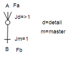
- Another way to look at it, that Dan Tow uses, is to look at the join filters.
- Where Jd, ie join detail, is the average number of rows returned when join in a for from the master.
- Likewise Jm is the master join ratio or the average number of rows that are returned joining from the child into the master. Generally speaking the Jm will be 1 in the case of PK/FK relations, though it might be smaller for unique indexes or unique constraints on the master join column instead of PK/FK.
- In rare cases if the join into the the detail can return less than 1 on average, then in this case, it is just as good to join up to the "detail" as down to the master.
- NOTE: for minimum values returned, unless there is a constraint, a join can return 0 rows. A PK/FK relation will constrain that there be a parent(master) for each child(detail).
- All and all, I think the easiest route is just to display the join set sizes from each two way join.
Step 7: Table Sizes
- Finally, and maybe actually least, we can display the number of rows in a the tables in the query.
